
StreamCat Data Processing and Quality Assurance
Introduction
This document describes the main steps that we followed to develop the StreamCat Dataset, including quality assurance (QA) procedures.
Processing and QA Steps
Here we outline the steps we took to process the raw data and assure quality standards throughout the different stages of this project.
1. Landscape Layer Acquisition
The development of the StreamCat Dataset is a part of a multi-phased project. For the first phase of this project, we identified potential landscape metrics through a literature review. Specifically, we used several landscape metrics identified in Carlisle et al. 2009, Falcone et al. 2011, and Wang et al. 2011. Data were downloaded from online sources where available. Some layers (e.g., STATSGO Soils layers) were obtained directly from James Falcone of the USGS.
For the second phase of this project, we conducted an extensive search for publicly available, conterminous USA-wide landscape layers that we hypothesized could improve our representation of natural and anthropogenic watershed features. These layers included climate, groundwater usage, forest cover change (yrs. 2001-2010), atmospheric N deposition, and fish passage barriers. These data will be added to this FTP site as they become available.
2. Layer Checks
The original characteristics of each landscape layer were documented and checked for consistency:
- Landscape Feature - Name of GIS layer used in analysis
-
Description - A short description of the landscape layer (see also Data Dictionary)
-
Source - From where the data were obtained, especially through personal contacts
-
Original GIS Format - Original file type of landscape layer
-
URL - URL from which layer was downloaded, if applicable
-
Check Projection - Check the original projection of the data. Desired projection was USGS Albers Equal Area Conic Projection
-
Check raster resolution - Documentation of the resolution of GIS raster, if applicable
-
Check Spatial Extent - Verify that the raster covers the conterminous USA (visual check)
-
Crosses CAN/MEX borders - Check whether layer extends into Canada or Mexico
-
Check NoData Values - For raster layers, document the NoData values (e.g., -9999 vs. true NoData values)
-
Check Units - Document the units of data layers, if applicable
-
Visual Check - Opened layer in ArcGIS and visually inspected it for outliers, odd values, file corruption
3. Layer Manipulation
After documenting the original characteristics of each dataset, we then manipulated the data to standardize geospatial projections and other characteristics across layers where necessary. Data were standardized using a Python script, StandardizeLandscapeFeatures.py. Manipulations, final data formats, and final data units were documented, including:
- Unit or NoData Conversion - ArcGIS raster calculator commands to convert to SI units
- Final Units - The final units of layers, if applicable
- Check range of converted values - Verify that values of final layers are within expected ranges
- Final GIS Format - The final file type of landscape layer
- Notes - Additional notes and actions that were required to standardize landscape layers
4. Zonal Statistics Geoprocessing
The first step to create watershed metrics was to generate statistical summaries of landscape layers for each catchment. We overlaid the catchment boundaries onto landscape layers and calculated a suite of summary statistics (Table 1). Raster layers were processed using a Python script, zonal_stats.py. Point or line features were processed using an R script, ZonalStatsProcessing.Rmd.
Table 1. Example of a zonal processing results for a continuous raster type. Results differed from this example if original landscape layer was a categorical data type.
| FEATUREID | COUNT | AREA | MIN | MAX | RANGE | MEAN | STD | SUM |
|---|---|---|---|---|---|---|---|---|
| 179 | 3950 | 3555000 | 14.0495 | 14.3705 | 0.3209991 | 14.35465 | 0.0695391 | 56700.8786 |
| 181 | 322 | 289800 | 14.3705 | 14.3705 | 0.0000000 | 14.37050 | 0.0000000 | 4627.3009 |
| 183 | 227 | 204300 | 14.3705 | 14.3705 | 0.0000000 | 14.37050 | 0.0000000 | 3262.1034 |
| 185 | 41 | 36900 | 14.3705 | 14.3705 | 0.0000000 | 14.37050 | 0.0000000 | 589.1905 |
| 843 | 3054 | 2748600 | 17.6645 | 19.5475 | 1.8830013 | 18.49687 | 0.9351543 | 56489.4326 |
| 845 | 4274 | 3846600 | 19.5475 | 19.5475 | 0.0000000 | 19.54750 | 0.0000000 | 83546.0176 |
5. Catchment Results Cleanup
Step 4 produces statistical summaries that are stored in .dbf files. Next, we selected and renamed a subset of columns from these dbf files and placed them into new, comma delimited files (Table 2). The subset of columns that are contained in the new file depends on the type of base landscape layer (raster, point, line) and whether the watershed metric is based on a continuous (e.g., soils) or categorical (e.g., land cover) data type. In addition, the area (km2) of catchments is appended from the NHDPlusV2. This step was processed with an R script, ZonalStatsProcessing.Rmd
Table 2. Example of a cleaned catchment results for a continuous raster type. Results differed from this example if original landscape layer was a categorical data type.
| COMID | CatAreaSqKM | CatMean | CatPctFull | CatCount | CatMin | CatMax | CatRange | CatStd | CatSum |
|---|---|---|---|---|---|---|---|---|---|
| 179 | 3.5550 | 14.35465 | 100 | 3950 | 14.0495 | 14.3705 | 0.3209991 | 0.0695391 | 56700.8786 |
| 181 | 0.2898 | 14.37050 | 100 | 322 | 14.3705 | 14.3705 | 0.0000000 | 0.0000000 | 4627.3009 |
| 183 | 0.2043 | 14.37050 | 100 | 227 | 14.3705 | 14.3705 | 0.0000000 | 0.0000000 | 3262.1034 |
| 185 | 0.0369 | 14.37050 | 100 | 41 | 14.3705 | 14.3705 | 0.0000000 | 0.0000000 | 589.1905 |
| 843 | 2.7486 | 18.49687 | 100 | 3054 | 17.6645 | 19.5475 | 1.8830013 | 0.9351543 | 56489.4326 |
| 845 | 3.8466 | 19.54750 | 100 | 4274 | 19.5475 | 19.5475 | 0.0000000 | 0.0000000 | 83546.0176 |
6. Metric Accumulation & QA
Catchment results were accumulated to produce watershed-level summaries of landscape metrics for all ~2.65 million NHDPlusV2 streams and associated catchments. The accumulation algorithm is described in Hill et al. (in review). Accumulations were executed using a Python script, CatchmentAccumulation.py. This script accesses functions available in SpatialPredictionFunctions.py.
Accumulation results were saved in comma delimited (.csv) text files. These tables contained summary statistics of landscape layers for each catchment as well as the upstream, accumulated catchments (Table 3). Note that the upstream accumulations did not include catchments summaries in them. In the example table below, columns 2 - 5 contain information for the catchments identified by the COMID (column 1). Columns 6 - 10 contain information on the upstream catchments flowing to the catchment, excluding the catchment. In this example, COMID 179 is a headwater catchment because its 'Up' results are all 0s.
Table 3. Example of an accumulation results for a continuous raster type. Results differed from this example if original landscape layer was a categorical data type.
| COMID | CatAreaSqKm | CatMean | CatPctFull | CatCount | CatSum | UpCatAreaSqKm | UpCatMean | UpCatPctFull | UpCatCount | UpCatSum |
|---|---|---|---|---|---|---|---|---|---|---|
| 179 | 3.5550 | 14.35465 | 100 | 3950 | 56700.8786 | 0.0000 | 0.00000 | 0 | 0 | 0.00 |
| 181 | 0.2898 | 14.37050 | 100 | 322 | 4627.3009 | 3.5550 | 14.35465 | 100 | 3950 | 56700.88 |
| 183 | 0.2043 | 14.37050 | 100 | 227 | 3262.1034 | 7.9911 | 13.64091 | 100 | 8879 | 121117.65 |
| 185 | 0.0369 | 14.37050 | 100 | 41 | 589.1905 | 8.1954 | 13.65910 | 100 | 9106 | 124379.76 |
| 843 | 2.7486 | 18.49687 | 100 | 3054 | 56489.4326 | 0.0000 | 0.00000 | 0 | 0 | 0.00 |
| 845 | 3.8466 | 19.54750 | 100 | 4274 | 83546.0176 | 6.5394 | 19.01572 | 100 | 7266 | 138168.22 |
We conducted a QA check on these tables to ensure that the scripts were producing the correct number of records and correctly accumulating data. Correct results in this QA check also indicated that we were successfully processing steps 4 and 5. Among these checks, we compared the number of records and watershed areas in the accumulation results to those in NHDPlusV2. All records were an exact match except a single watershed in HydroRegion 07 that was 0.162 km2 smaller than the same record in NHDPlusV2 (Table 4).
Table 4. Example results of QA check. Checks were conducted for all regions and all processed variables. The first check verified that the accumulation process produced the same number of catchments as contained in each of the NHDPlusV2 regions. The second check compared StreamCat and NHDPlusV2 accumulated watershed areas and recorded the number of records that were not an exact match.
| RegionID | MissingResults | AreaMisMatches |
|---|---|---|
| 1 | 0 | 0 |
| 2 | 0 | 0 |
| 03S | 0 | 0 |
| 03N | 0 | 0 |
| 03W | 0 | 0 |
| 4 | 0 | 0 |
| 5 | 0 | 0 |
| 6 | 0 | 0 |
| 7 | 0 | 1 |
| 8 | 0 | 0 |
| 9 | 0 | 0 |
| 10L | 0 | 0 |
| 10U | 0 | 0 |
| 11 | 0 | 0 |
| 12 | 0 | 0 |
| 13 | 0 | 0 |
| 14 | 0 | 0 |
| 15 | 0 | 0 |
| 16 | 0 | 0 |
| 17 | 0 | 0 |
| 18 | 0 | 0 |
To date, we have not been able to identify the sources of this difference for COMID 2456642. In addition, our accumulated areas exactly match the NHDPlusV2 watershed areas directly upstream and downstream (COMIDs 2456374 and 2456640) of this record (Figure 1).
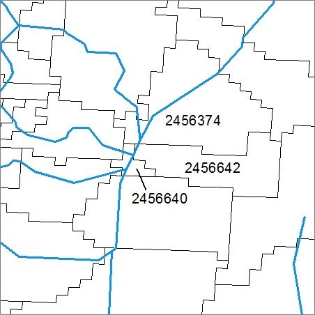
Figure 1. Catchments 2456642, 2456374, and 2456640 in HydroRegion 07. StreamCat-NHDPlusV2 comparison of areas identified a 0.162 km2 difference for COMID 2456642.
7. Final Tables
Final tables were produced for distribution from the accumulation tables (step 6). To produce final tables, we combined "Cat" results with "Up" results to produce full watershed ("Ws") summaries of landscape features. Final tables are available via our public API or through the Map and Table tools.
Tables were produced with an R script, FinalTables.Rmd . The set of features contained in final tables depended on the original landscape layer being summarized. In addition, some metrics from common data sources were combined in final tables, such as STATSGO Clay and Sand content of soils. Summaries of landscape metrics are provided in individual metadata files and in the data dictionary. Tables contain a unique identifier (COMID, column 1) that can be related back to the NHDPlusV2 streams and catchments shapefiles. After the COMID, ancillary information is provided, including the area of the catchment (km2), the % of the catchment that overlapped with the landscape layer (i.e., accounting for NoData values and international borders), the area of the watershed (km2), and the % of the watershed that overlapped with the landscape layer. Following ancillary information, catchment ("Cat") and full watershed ("Ws") summaries of landscape metrics are provided.
Table 5. Example of a final table for a continuous raster type. Results differed from this example if original landscape layer was a categorical data type.
| COMID | CatAreaSqKm | CatPctFull | WsAreaSqKm | WsPctFull | ClayCat | SandCat | ClayWs | SandWs |
|---|---|---|---|---|---|---|---|---|
| 179 | 3.5550 | 100 | 3.5550 | 100 | 14.35465 | 22.33890 | 14.35465 | 22.33890 |
| 181 | 0.2898 | 100 | 3.8448 | 100 | 14.37050 | 22.33238 | 14.35585 | 22.33840 |
| 183 | 0.2043 | 100 | 8.1954 | 100 | 14.37050 | 22.33238 | 13.65910 | 23.55634 |
| 185 | 0.0369 | 100 | 8.2323 | 100 | 14.37050 | 22.33238 | 13.66229 | 23.55085 |
| 843 | 2.7486 | 100 | 2.7486 | 100 | 18.49687 | 20.60167 | 18.49687 | 20.60167 |
| 845 | 3.8466 | 100 | 10.3860 | 100 | 19.54750 | 20.12630 | 19.21267 | 20.27779 |
We verified the results of the final tables by comparing accumulated precipitation (continuous data type) and NLCD 2011 (categorical land cover data) values with precipitation and NLCD 2011 data distributed by NHDPlusV2. For this check, we obtained the precipitation raster directly from Horizon Systems, Corp. In most cases, our precipitation values were within 0.005 mm of the NHDPlusV2 values (Figure 2). In cases where differences were >0.005 mm, we were able to account for why these differences occurred. See the Precipitation QA Check for additional details regarding the results of this QA check.
Similar results were found for most NLCD 2011 comparisons. However, differences in catchments that cross international borders were noted due to the different methods used to develop the StreamCat Dataset and NHDPlusV2 Data Extensions.
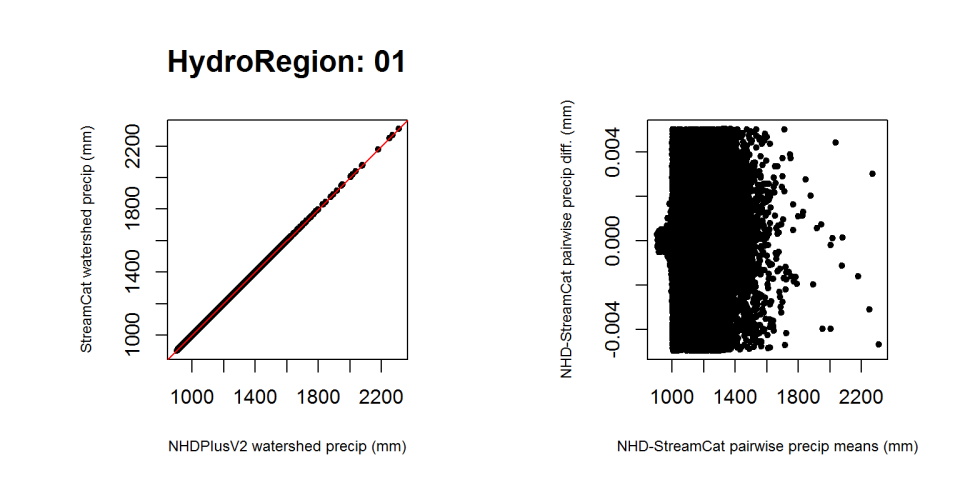
Figure 2. Example comparison of StreamCat and NHDPlusV2 precipitation values. Differences were typically between -0.005 and 0.005 mm