Mechanistic Modeling

In 2000 and 2001, EPA released a series of peer-reviewed technical guidance documents for developing nutrient criteria for lakes and reservoirs, rivers and streams, and estuarine and coastal marine waters. The documents outline three types of analysis for deriving numeric criteria: (1) the reference condition approach, (2) mechanistic modeling, and (3) stressor-response analysis. This page provides an overview, with four successive pages that provide more detail on mechanistic modeling and how states can use mechanistic models to derive numeric nutrient criteria. Mechanistic models are used in a number of applications related to nutrient criteria including development of total maximum daily loads (TMDLs), watershed improvement plans, determining background conditions, and developing site-specific criteria. For more comprehensive model information, consult textbooks and user manuals for models.

Mechanistic Water Quality Models are Mathematical Representations of Environmental Processes

Mechanistic models describe water movement in one two or three spatial dimensions; the physical, chemical, and biological processes in the water; and the interactions of all of these properties coupled with water movement. They are based on the laws of conservation of momentum, heat energy, water mass, and contaminant mass. The laws of conservation of mass and of momentum are the basis for the equations for water movement, or hydrodynamics. Conservation of mass and heat are applied to water quality constituents and temperature. Mechanistic models are able to represent the transport and fate of nutrients and the functional relationship between nutrients and algae production.

Each set of mathematical equations relates something unknown—such as water quality response—to some measureable data—such as precipitation, land use, and nutrient loadings. While mechanistic models are used when historical observed data records are not available, are too short, or are otherwise inappropriate for reliable statistical analysis, the power of mechanistic models is they can be used to predict the response of an ecosystem to changes in environmental stressors (e.g., loads or flows). 

Mechanistic models provide a way to predict flow, velocity, timing, and water quality to inform management decisions to prevent degradation of water quality or to restore polluted waters. In contrast to the reference condition approach—which relies on water bodies to be minimally impacted or unimpaired—mechanistic modeling has no such requirements. The models can be configured to match the existing condition—either high-quality or low-quality waters—and used to predict the changes necessary to attain the desired water quality condition. Mechanistic water quality models were developed to further the understanding of the levels of discharged pollutant loads that result in a desired condition in the receiving water. Scientists and engineers have added more processes to the models over time, and their popularity as a tool in water quality management has grown. For example, mechanistic water quality models are widely applied to developing TMDLs and water quality-based effluent limits for permits.

Mechanistic models are primarily categorized by pollutant (e.g., nutrient, sediment, etc.), water body type (e.g., ground water, river system, coastal waters, etc.), steady-state or dynamic, and dimension (1 dimensional [1-D], 2-dimensional [2-D], or 3-dimensional [3-D]). The primary functional types of models are watershed models, hydrodynamic models, and water quality models.

In general, to derive nutrient criteria, models need to be configured, calibrated, and validated. Then, nutrient loading inputs are adjusted until the model predictions match the desired water quality conditions. The resulting, simulated condition is similar to a reference condition in which designated uses are attained and is the condition from which criteria are derived.

Benefits of the Mechanistic Model Approach

Mechanistic models can be used to:

• Predict changes in a water system, given changes in nitrogen and phosphorus concentrations due to land use changes, BMP implementation, NPDES load reductions/increases
• Provide insight and understanding to water quality problems
• Evaluate downstream effects
• Ensure that results are defensible and credible

Because mechanistic models describe environmental processes and interactions, they can be used to predict responses, provide insight, and evaluate downstream effects. For example, Nutrient criteria developers can use models to predict changes in a water system, given changes in nitrogen and phosphorus concentrations associated with changes in point or nonpoint source loadings to the water system. The criteria developer can apply the models to simulate conditions that will result in desired levels of algal biomass, water clarity, dissolved oxygen (DO), and other measures of designated use attainment. You then can use the simulated concentrations of nitrogen, phosphorus, and chlorophyll a to derive nutrient criteria. Criteria developers also can use the models to simulate scenarios in which corresponding empirical data are not available.

Mechanistic models provide insight into and understanding of water quality problems, such as analyzing various environmental components to see which processes impact a variable of interest. Criteria developers can analyze various environmental components to see which processes impact a variable of interest. For example, to analyze DO, mechanistic models are used to examine each of the mechanisms that affects DO to see how much oxygen is consumed by each of the processes. Specifically the models can be set up to evaluate sediment oxygen demand (SOD) and biochemical oxygen demand (BOD) processes and how much oxygen is produced by algae. The result provides information on which process has the greatest effect on the variable of interest.

Mechanistic models can be applied to individual water bodies, such as lakes, reservoirs, or estuaries, or groups of connected waters such as a chain of lakes, system of reservoirs, or watershed system. For example, the criteria developer can calibrate a hydrodynamic and water quality model to site-specific conditions in an estuary to represent that system, and then derive nutrient criteria. You could use that same model to determine nutrient levels for each tributary stream that results in meeting the estuary criteria. In that way, the model provides a tool you can use to evaluate downstream effects of the stream water quality on the estuary. The criteria developer also could use a watershed model in conjunction with an estuary model to evaluate the water quality within the watershed streams.

Another feature of mechanistic models that is important to the regulatory environment of nutrient criteria development is providing a peer-reviewed and widely used framework that is credible and defensible. Since each model is a collection of mathematical equations, it is a structure or framework that you can tailor to a particular water body and review easily. The framework also allows for review of the parameterization of kinetic processes (which are represented by the mathematical equations in the model), evaluation of data used for the model, evaluation of assumptions made, and review of of the calibration process and results. The modeling framework organizes the information for these critical steps for easy review.

Types of Mechanistic Modeling

Here we focus on nutrient and eutrophication surface water quality models simplified into the primary functional types:

• Watershed models
  • Describe the hydrologic mechanisms and the delivery of contaminants from the watershed, specifically the land surface, to a stream, river, lake, or estuary.
  • Describe water movement and water quality processes on land and instream.
• Hydrodynamic models
  • Describe water movement within a water body in detail and in multiple directions.
  • Can describe the water movement in one, two, or three dimensions over a specified time period.
• Water quality models
  • Describe the changes that contaminants go through within a water body.
  • Do not simulate watershed processes, so pollutant loads must be provided to these models using results from a watershed model or measured data.
  • Can be linked with a hydrodynamic model, which will supply water movement information.
  • Can describe nutrient cycles, light attenuation, growth of algae, and production and consumption of DO (eutrophication models).
  • Can describe other related processes useful in nutrient modeling including submerged aquatic vegetation (SAV) dynamics, pH dynamics, and sediment diagenesis (movement of nutrients from the sediments to the water column).

Often models are used together. For example, a watershed model can provide tributary flows to a receiving hydrodynamic model, which then can provide water body hydrodynamics to a water quality model and the watershed model providing constituent loads to the receiving water quality model. Table 1 provides a list of commonly applied mechanistic models.

Table 1. Commonly applied mechanistic models

Model	Version	Date	Type	Dimension	Typical Uses
CE-QUAL-RIV1	3.0	11/1995	Hydrodynamic and water quality	1-D	Predicting 1-D hydraulic and water quality variations in streams and rivers  in both steady and unsteady flows
DYNHYD	5.0	9/1993	Hydrodynamic	1-D	Simulates tidal cycles, wind, and unsteady flows; supplies flows and volumes to WASP water quality model
EFDC	1.01	9/2007	Hydrodynamic	1-D, 2-D, 3-D	Studies of inflow events, discharge dilution, salinity intrusion, sediment transport, contaminant transport and fate, and water quality eutrophication
EPD-RIV1			Hydrodynamic and water quality	1-D	Analyzing existing conditions, performing waste load allocations, including TMDLs
HSPF	11.0	3/1997	Watershed hydrology and water quality	1-D	Contaminant transport and fate, water quality planning, flood control planning, storm drainage analyses, evaluation of BMPs, pollution management
LSPC	3.1	12/2009	Watershed	NA	Simulating hydrology, sediment, and water quality on land and simplified stream fate and transport; used for mining applications and TMDLs
SWAT	2012.659	9/2016	River basin hydrology	NA	Assessing soil erosion prevention and control, pollution control and regional management in watersheds
WASP	8.0	11/2016	Water quality	1-D, 2-D, 3-D	Studies of eutrophication and pollution, development of TMDLs and numeric nutrient criteria
QUAL2E			Water quality	1-D	Water quality planning, development of TMDLs
QUAL2K	2.12b1	2015	Water quality	1-D	Eutrophication studies, development of TMDLs, determination of environmental capacities in water bodies
ICM	7.5	12/2016	Hydrodynamic	1-D, 2-D	Drainage and sewer planning, surface water management, storm water runoff control design, hydraulic analysis of wastewater treatment facilities

Watershed Models

Developing nutrient criteria requires an understanding of the relationships between nutrients and various ecological responses. The underlying goal of the criteria is to manage nutrients that enter our water systems so the uses of lakes, rivers, and estuaries are not degraded. Nutrients can enter a water body in runoff from the land surface directly from rain or the air, and in ground water inflow, as well as from the sediments within the water body. Watershed models simulate the processes on the land and delivery of pollutants to the surface water system. You can use a watershed model to simulate nutrient management actions on land use, such as agricultural and urban stormwater best management practices (BMPs).

The degree of detail that can be included in the models varies greatly from one model to another, and the various commonly used watershed models offer several advantages and disadvantages. Simplistic models, specifically BATHTUB and WARMF, require comparatively little data input and can be set up using data available from government agency websites. The complexity of model setup also can depend on the overall size of the area of concern and the input spatial resolution desired. SWAT, HSPF, and LSPC are capable of simulating hundreds to thousands of subbasins and are highly adaptable to specific project needs through their incorporation of several watershed, water quality, and transport modules. SWAT, which was developed by the U.S. Department of Agriculture, is best suited to model rural and agricultural watersheds because model components focus on simulating vegetation dynamics and agricultural BMPs. Both HSPF and LSPC are slightly more data-intensive that SWAT and are better suited to simulating hydraulics and watershed loading in urban areas. Another model, SWMM, works well in urban-only areas because it can simulate the complex flow routing of urban drainage networks and evaluate flow and load reductions from low impact development controls, including infiltration trenches, green roofs, and permeable pavement. It cannot simulate, however, the complex instream nutrient-related biotransformations that SWAT, HSPF, and LSPC are capable of simulating.

The strengths of watershed models are their ability to estimate natural or undeveloped conditions to use as a lower bound for criteria development, as well as the effect of various nutrient management practices. While neither of these strengths is required for developing criteria, ;they are valuable for associated efforts such as TMDL development, permitting, and identification of the most appropriate nutrient management practices. A watershed model also can be used to determine nutrient levels within tributaries that result in attaining the downstream receiving water criteria (i.e., downstream protection).

Hydrodynamic Models

Flow is a key mechanism in water quality models, telling us where the water goes, and how fast it moves. Water movement affects delivery of contaminants and the concentrations of dissolved and suspended contaminants. Formulations for modeling water movement range in complexity from simplified 1D steady-state transport models to more complex multi dimensional and fully unsteady flow models.

The simplest model is a completely mixed system with constant flow and volume, and this steady-state condition can model some lakes (Chapra 2008; Martin and McCutcheon 1999). You also can model a river with EPA’s QUAL2E and QUAL2K models using a string of completely mixed systems. This simple 1-D river model adds equations for stream velocity, depth, and dispersion. However, most natural systems do not have a constant flow. Although steady-state models are simpler to configure, require less data, have shorter model run times, and generate less model output to analyze, they also require the modeler to determine a flow condition that can be used to develop water quality criteria. Determining these water quality critical conditions for a water body can be difficult because environmental flows, concentrations, and loadings vary over time and space. Also, pollutants such as nutrients accumulate over time and often cause responses far from the source and long after delivery. For these reasons, unsteady flows are often modeled.

One simple form of the unsteady flow equations is the kinematic-wave model, which is limited to one dimension and, therefore, can run relatively quickly. It cannot, however, be applied in systems in which downstream controls (such as dams) strongly influence the flow. Kinematic-wave models are commonly used and found in watershed models such as , a receiving water model (i.e., it receives the watershed loads or hydrodynamic flows from another model or from measured data; we typically call lakes and estuaries receiving water models), also includes options for kinematic-wave routing.

Full unsteady flow models solve the complete continuity and momentum equations, which can handle downstream controls such as dam backwater and ocean tides. They can be solved in one dimension (longitudinally) using DYNHYD, CE-QUAL-RIV1, and EPD-RIV1 models. Models such as CE-QUAL-W2 solve these equations in two dimensions (longitudinal and vertical), and EFDC solves the hydrodynamic equations in three dimensions. Both of these models also can be used to simulate one-dimensional (1-D) flows as well. James Martin and Steven McCutcheon’s Hydrodynamics and Transport for Water Quality Modeling (1999), and Terry Sturm’s Open Channel Hydraulics (2001) provide more detailed discussion of the water quality mechanisms included in models.

If there is good measured flow and water quality data upstream of a riverine area of interest, you can use receiving water models such as WASP and EFDC instead of a watershed model to evaluate changes in instream water quality. Receiving water models are typically less data- and process-intensive than watershed models (i.e., they do not need soils or land use data input, do not need to calibrate land use loadings) and, by eliminating the need for a watershed model, can be used at significant time and cost savings. In addition, both WASP and EFDC have more advanced eutrophication kinetics than the watershed models and have coupled sediment diagenesis modules. For example, WASP and EFDC can represent three types of phytoplankton compared to only one type represented in watersheds, which you can use to simulate multiple phytoplankton blooms over the period of a year.

Water Quality Models

For numeric nutrient criteria development, models that relate nutrients to an assessment endpoint, such as eutrophication, are needed. HSPF, LSPC, and QUAL2E include basic eutrophication processes, and CE-QUAL-ICM and WASP7 include eutrophication processes with advanced options. These models can include nutrient cycling, algal growth, light mechanics, and DO dynamics. In some cases, simple models are used to evaluate nutrient changes in time, often along a 1-D pathway such as length of a flow path in a stream or in 2-D as the area of a lake. A simple model might include a constant SOD, single phytoplankton group, and simple light mechanics. A more complex model might include several light attenuation components such as algae, suspended solids, and colored dissolved organic matter. In water systems in which SOD plays a major role in the DO deficit, modeling the changes in SOD that correspond to changes in nutrient loading might be necessary. SOD is modeled with sediment diagenesis models, which compute the mass balance of settling particulate organic matter, reactions within the sediments, and concentrations of soluble nutrient forms in the overlying waters. Water quality models with sediment diagenesis routines include CE-QUAL-ICM, EFDC, and WASP. In some systems, understanding the different spatial and temporal dynamics in phytoplankton functional groups might be important, and modeling two or three algal groups such as diatoms, green algae, and cyanobacteria is necessary. Benthic algae also can be an important component of water systems such as shallow portions of rivers and streams and clear estuaries and a useful assessment endpoint. Many commonly used models do not have benthic algae routines, but more comprehensive models such as CE-QUAL-ICM, QUAL2K (Chapra et al. 2008), and WASP7 (Ambrose et al. 2006) are incorporating modeling routines for benthic algae. In addition to benthic algae, CE-QUAL-ICM includes routines for SAV (roots and shoots biomass) and epiphytes. Another property influenced by eutrophication is pH, and significant changes in pH can negatively impact aquatic life. Because pH has historically been associated with metals and toxicity modeling, many eutrophication models such as EFDC, ICM, and the WASP eutrophication model do not include pH; however, some models such as QUAL2K and WASP advanced eutrophication version 8.0 do include pH.

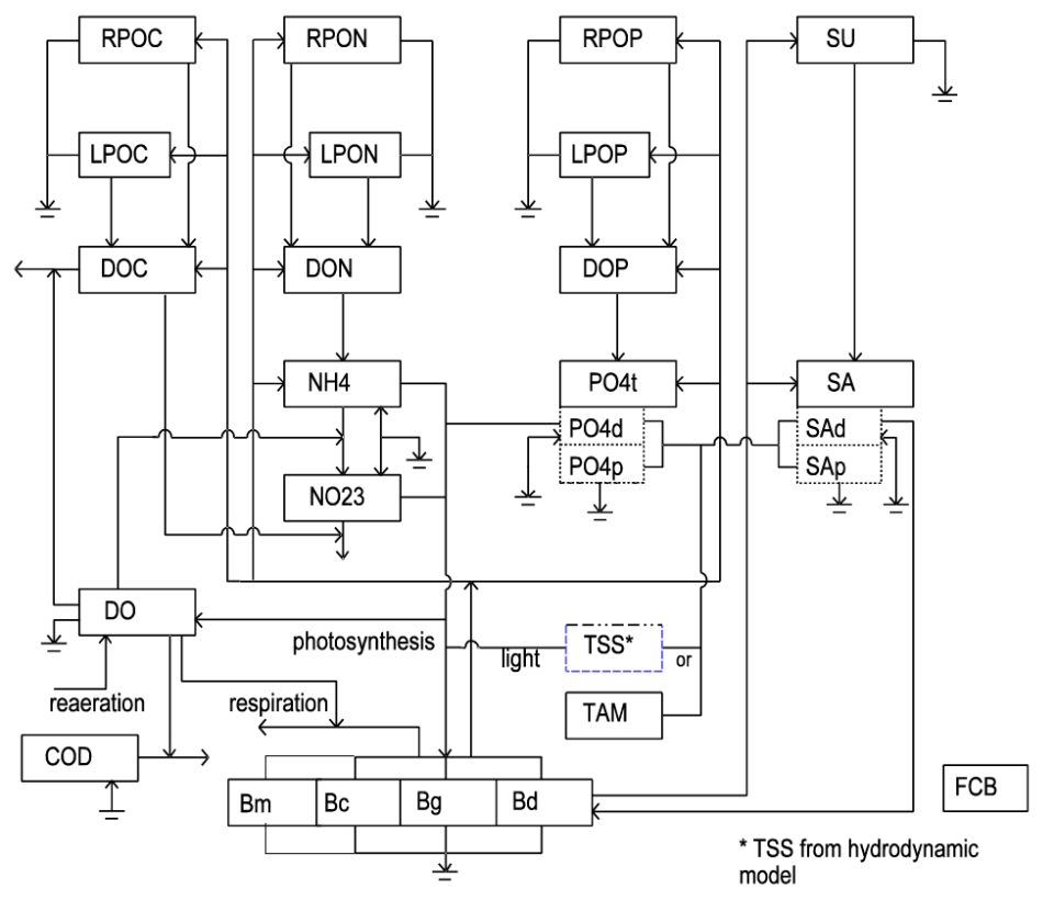
Water quality models can be very complex and take into account numerous processes that are occurring in a water body. Figure 1 illustrates the complex nutrient cycling that occurs in the EFDC model, specifically how those processes impact primary production and dissolved oxygen (DO) concentrations. The model simulates 21 state variables, including the exchange of fluxes at the sediment-water interface, such as sediment oxygen demand.

More details about the water quality mechanisms included in models can be found in EPA’s Rates, Constants, and Kinetics Formulations in Water Quality Modeling (Bowie et al. 1985), model user manuals, and many texts such as Steven Chapra’s Surface Water-Quality Modeling (1997) and Robert Thomann and John Mueller’s Principles of Surface Water Quality Modeling and Control (1987).

Simple Models

There are a number of simple water quality models that are available to help provide additional lines of evidence for a criteria development process or to check some assumptions. For example, there are some simple lake loading models that evaluate the input, accumulation, and outflow of a single nutrient to a system. Some examples of these types of models are described. The first model predicts trends in nutrient accumulation of a lake; phosphorus is used to illustrate the nutrient dynamics in this example. The second example shows periphyton growth in streams.

Lakes

Simple mass balance models could focus on characterizing major inputs and outputs to predict the long-term trends of a lake’s response to loading changes.

The simplest example of a total phosphorus (TP) budget model was developed by Vollenweider (1968) and modified by Chapra (1975):

As depicted in Figure 2, the key feature of this model is the simple way in which it characterizes the input-output terms for TP. The model characterizes sedimentation losses as a simple one-way settling of TP (a) and settling with burial and recycling of phosphorus components (b).

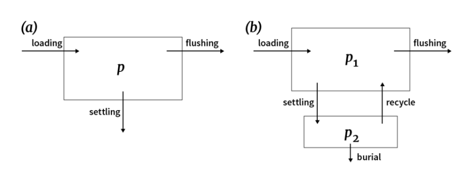
Models like the one shown in Figure 2 can be used for steady-state or dynamic scenarios. Steady-state solutions can be developed by setting the derivative to 0 and solving for p = W/(Q + vA). If levels of TP can be associated with a trophic state, the criteria developer can use the model to determine the loading required to maintain a particular lake at a desired quality in a fashion similar to empirical phosphorus loading plots (Chapra 2008). The model also provides a framework you can use to determine the temporal response of a lake to loading changes.

Phosphorus budget models have been improved in several ways. For incompletely mixed systems, the lake can be divided into a system of interconnected well-mixed systems either horizontally or vertically. For example, Chapra (1979) used two mass balances to characterize a lake with a major embayment. In a similar manner, O’Melia (1972) and others have vertically divided the water column of thermally stratified lakes into surface and bottom layers.

For lakes and reservoirs efforts have been made to better characterize sediment–water interactions. Chapra and Canale (1991) represented a lake and its underlying sediments as a two-layer system. Along with phosphorus settling, this model also allows sediment feedback (Figure 2(b)). A simple oxygen model is used to simulate hypolimnetic anoxia, which triggers sediment release of TP into the overlying waters. This mechanism is significant because sediment feedback can hinder the recovery of lakes after TP load reductions. Hybrid models have been developed that use mass balance and multiple segments to characterize transport. To quantify kinetics, they use empirically derived relationships. Walkers BATHTUB model for reservoirs is a good example of this type of model.

In summary, phosphorus budget models use simple mass balance to characterize how phosphorus levels change in lakes in response to load modifications. Thus, the assumption is made that “as goes phosphorus, so goes eutrophication.” These models can be useful for simulating the long-term trends in the quality of phosphorus-limited lakes and reservoirs.

Streams

Chapra et al. (2014) developed a simple, process-based model to assess the impact of nutrients on shallow, periphyton-dominated streams. The model builds on a simple model of available nutrients and bottom algae from Thomann and Mueller (1987) and has a minimal number of parameters. You can use it to predict periphyton biomass based on available phosphorus concentration, nitrogen concentration, light, and temperature. Periphyton biomass (mgAm−2), a(x), at distance x downstream:

Constant temperature and light levels are assumed. Additional model conditions include steady-state, uniform conditions (i.e., constant parameters) and nutrient concentrations at the mixing point well above saturation. Given reasonable parameter estimates, the following equation provides a way to establish a model-based nutrient criterion:

Checklist for Success

Select models that can represent important flow dynamics and water quality processes

Modelers, scientists, and decision makers need to collaborate on selecting a model, or set of models, that can simulate the water movement and biological and chemical processes that cause the movement and cycling of nutrients in a water system. You should consider how the water moves in the water body and which type of model can most accurately represent that movement or circulation pattern. Additionally, the criteria developer should consider which nutrient-related biological, physical, and chemical processes are needed to represent the water body.

To help you select appropriate models for analyzing nutrients in surface waters, Water Environment and Reuse Foundation (WE&RF) has developed the Model Selection Data Toolbox.

Select models that represent the movement of the waterbody

One of the biggest advantages of using mechanistic models is being able to represent how the water moves within the water body. When selecting a model or set of models to address nutrient criteria, select a model that can simulate the movement of the water body. Models describe water movement in 1-D, 2-D, or 3-D spatial dimensions. You also can use them to represent water flow, velocity, and volume as remaining constant over time (steady-state) or as changing over time (dynamic).

Steady-State Model for Well-Mixed Lakes, Reservoirs, Streams and Rivers

Well-Mixed 1-D Kinematic-Wave Model

Well-Mixed 1-D River or Reservoir Fully Dynamic Flow Model

2-D Hydrodynamic Models

3-D Hydrodynamic Models

Select models that represent the water quality processes that are important

When selecting a model or set of models to address nutrient criteria, you need to represent the important water quality processes. For nutrient criteria, those processes include:

• Nutrient cycling
• Algal growth
• Light mechanics
• DO dynamics
• Sediment diagenesis
• pH dynamics
• SAV dynamics

Some of the issues to consider include the following:

• Can one algal group represent the system or should multiple groups be modeled (e.g., greens, diatoms, and cyanobacteria)?
• Will DO be adequately represented with SOD as a constant rate or should sediment diagenesis be modeled?
• Are sediment interactions with the water column important?

Consider Temporal Variability

Consider the temporal variability when selecting a model for nutrient criteria development. If temporal variability is not important, or the model is applied for worst case conditions, then steady-state models can represent a useful alternative for the problem. If temporal variability is important for the problem, for example in applications requiring an accurate representation of daily cycles of production – respiration during different seasons, then a fully dynamic model must be consider. Models can be divided into steady-state and time-variable. Pollutant discharges, stream flows, and designated use impacts can vary markedly over time as a result of precipitation and runoff and seasonal effects on plant growth. In a time-variable model, external parameters such as inflows and loadings change with time, and the response to those changes are predicted. When selecting a model, you need to decide whether to develop criteria by evaluating a single condition or varying conditions. By considering a critical condition, you could derive criteria using a relatively simple steady-state model.

Most natural systems do not have a constant flow and, therefore, to use a steady-state model, you need to select a flow condition that represents a critical condition in which nutrient pollution is likely to cause worst-case, undesirable responses. Water quality criteria developed for a critical condition are protective of all, less severe conditions. Determining these water quality critical conditions for a water body can be difficult because environmental flows and pollutant concentrations vary over time and space. Additionally, pollutants such as nutrients accumulate over time and often cause biological responses long after delivery. A common critical period for nutrient impacts in streams is the summer low-flow, high-temperature period, which is favorable for nuisance plant growth. Often, a minimum 7-day average flow with a 10-year return period is used to determine water quality-based permit limits, and so this flow also could be applied as a critical condition. For example, the Montana Department of Environmental Quality conducted an analysis based on algal growth rates to justify a 14-day average flow condtion for nutrient NPDES permitting, and determined that a 5-year return period was a proper frequency. That analysis resulted in a 14-day average flow with a 5-year return period design condition for their steady-state nutrient criteria model of the lower Yellowstone River (MDEQ 2011). Critical conditions also can occur at other times of the year.  For example, in the fall, upstream organic carbon from decaying phytoplankton and aquatic plants can result in large depressions in DO levels.  Spring floods that pick up large amounts of organic debris from adjacent floodplains also can result in severe DO depletion or phytoplankton blooms (USEPA 1997). Another analysis approach is to evaluate several conditions independently. You could evaluate a summer low-flow condition, a spring high-loading condition, and a fall senescence condition. This concept is similar to civil engineers evaluating various flow conditions in bridge and culvert design.

Models used for steady-state simulations include the well-mixed stream or river steady-state models QUAL2E and QUAL2K. Alternatively, dynamic models can be used to obtain steady-state simulations by forcing them with constant boundary conditions. In summary, if a system is well-mixed and you can identify a critical condition, a steady-state model can be considered.

Alternatively, you can use a time-varying approach to determine the expected worst case for nutrient effects. With time-varying conditions, you should look at a number of high flows and low flows scenarios to represent high nutrient delivery and high water body retention times to make sure the full impacts of nutrient conditions are represented. Running the model for long periods, however, can take several hours or several days of computing time and generates large data sets, both of which can increase effort and expense. One way to address the long model runs is to calibrate and validate the model for multiple years, consider the results, and then pick the critical period to evaluate (e.g., 6 months or 1 year).

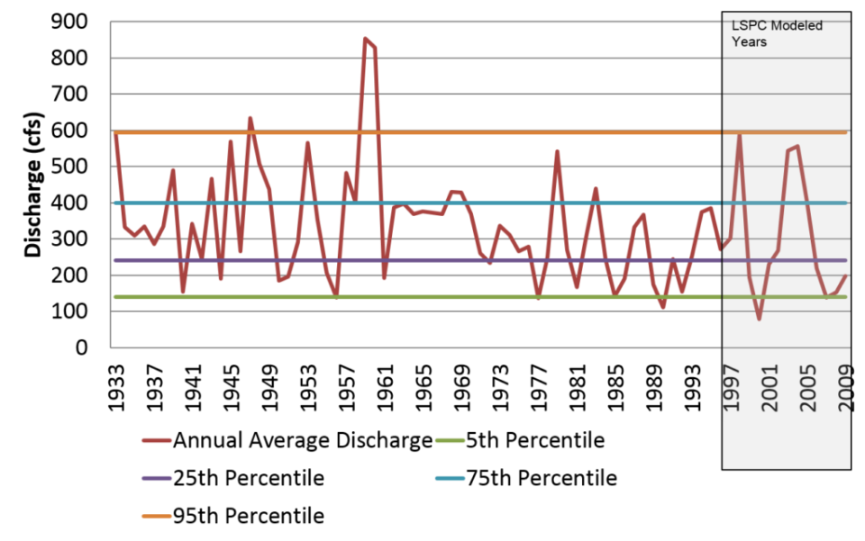
When selecting the modeling period for a time-varying simulation, consider hydrology, pollutant loadings, water quality data availability, and forcing function data availability. Figure 3 shows 75 years of flows at a gaging station and the 12 years used in a time-variable model. The modeling period was based on available data and hydrology representative of highs and lows discharged from the area being modeled. Nutrient concentrations and loadings can have patterns that are similar to or different than flow. Thus, analyzing the variations of all three  is important when considering a time-varying or steady-state approach. It is also helpful to consider expected future conditions to see if they are represented.

Additionally, when selecting a model, note that some models can be configured at either steady-state or dynamic state while other models can simulate only steady-state conditions.

Limitations of steady-state approach:

• Temporal changes in water quality cannot be evaluated e.g. Seasonal variability of DO and interdaily swings of DO in response to changes in phytoplankton production and respiration.
• Might not capture the biological effects that can lag behind the time when nutrient levels are elevated
• Does not account for spikes in nutrient levels followed by rapid nutrient uptake by algae and the resulting growth that can occur after ambient nutrient levels fall

Advantages of steady-state approach:

• Models run faster and generate less data to analyze at a lower cost
• Water quality data and forcing data for model configuration can be much easier to obtain for a single condition than for continuous period representing varying conditions

Limitations of dynamic-state approach:

• Requires more data, takes more time to configure and execute, and generates more data, which can increase analytical costs

Advantages of dynamic-state approach:

• Captures more realistic environmental conditions

Consider Spatial Extent and Scale

Spatial extent and scale must be addressed when selecting a model. Spatial extent pertains to the specific boundaries of the area to be assessed. Spatial scale refers to the number of dimensions to be considered and the degree of resolution (e.g., the model reach length, cell, or grid size) to be provided in each dimension. The degree of spatial variability and spatial extent are model configuration issues and are discussed in the model configuration topic. Spatial dimension is important to consider in model selection since it is specific to a model’s capability, and you should select a model capable of representing the necessary dimensions.

For example, real estuaries and near-shore waters all exhibit 3-D properties (e.g. circulation in the three spatial dimensions). There are gradients in hydrodynamic and water quality constituents over length, width, and depth. Thus, 3-D models are commonly used to model estuaries.

Table 2. Typical use of 1-D, 2-D, and 3-D models

Dimension	Typical Use and Considerations
1-D	Change in pollutant concentration over a single dimension in space, typically oriented longitudinally down the length of an estuary or lake
2-D	Concentration gradients in the lateral and longitudinal directions (x-y orientation)
3-D	Changes in concentration that occur over all three spatial dimensions The most detailed assessment of pollutant distribution with respect to a discharge The most extensive model input requirements and the most difficult to apply

Lakes and reservoirs are commonly modeled in 2-D or 3-D by assuming gradients in the vertical and/or lateral dimension are insignificant with respect to nutrient dynamics. For example, modeling a long, deep, narrow reservoir as a 2-D, laterally averaged system might be appropriate. Such reductions in dimensionality result in savings in model development, simulation time, and analysis costs. Rivers and streams are commonly modeled in 1-D or 2-D. Eliminating a spatial dimension from the water quality analysis implies acceptable uniformity of water quality constituents in that dimension. For example, use of 1-D longitudinal models, vertically and laterally averaged. That judgment requires an understanding of both the transport behavior of the water body and the specific objectives of the study.

Before selecting a model, you can determine the spatial variation in your water body by plotting observed water quality concentrations versus distance along the dimensions of concern. If such data are not available, vertical and lateral variations can be determined in one of several ways: density, salinity, or temperature gradients; tidal or velocity reversals over width or depth; dye cloud splitting and density-driven circulation; or geomorphological classification (USEPA 1990). If the water body is well-mixed vertically, the vertical dimension can be neglected, and all constituents in the water column are assumed to be dispersed evenly throughout. Be aware, however, that even though a water body can appear to be well-mixed in terms of temperature or salinity, it is still possible that water quality experiences a vertical gradient due to influences of the photic zone. Abundant light at the surface can cause higher algae and lower nutrient concentrations near the surface, and sediment diagenesis can cause higher nutrient concentrations near the bottom. These effects might not be completely offset by advective mixing. Commonly, in lakes and estuaries that are highly stratified and deep, the model may require several vertical segments to be able to capture the stratification patterns.

Key Challenges

• Data gaps
  • Some data are less expensive (e.g., DO, temperature), while others are more expensive (e.g., SOD, benthic flux rates)
  • Some data might be less likely to be representative of an entire waterbody or calibration period—this can negatively impact calibration
• Technical expertise
• Resources challenges—financial, time

Technical Requirements

You will need to configure the model to represent the important processes. The rates for nutrient cycling, algal growth, light mechanics, and DO dynamics include phytoplankton growth rate, death rate, and settling rate, and light attenuation factors for each component. It is difficult to obtain measurements for many of these rates. For example, to measure nutrient fluxes and sediment oxygen demand, divers must place a chamber on the water body bed surface and extract sample water from the chamber. Depending on the depth of the water body, visibility, and/or boat traffic, it might not be feasible to collect the samples. In addition, one set of flux samples costs approximately $2,000–4,000; therefore, if data is collected, it might be collected only once in key locations.

Typically, parameters that are more difficult to measure are estimated from literature values, data from neighboring water bodies, or previous modeling studies. If you plan to use parameters estimated from other data sources, it is best to work with stakeholders to make sure they agree with the data sources. During calibration, these kinetic rates are adjusted, and you should adjust them to fall within the range of known values.

If your stakeholders or you, however, are concerned about specific parameters, such as those to which the model is most sensitive, you might need to collect additional data. It is best to identify those parameters prior to modeling and develop a sampling plan for them. Before you develop the model, you should review the available data and determine what data are available for boundary conditions, calibration, and kinetic rate and constants. Collecting more data to fill the gaps can greatly improve model results and stakeholder buy-in. You will need to determine where and how frequently to collect samples. For some data, such as algal growth, it is best to collect samples at a high frequency over an entire growing season. In addition, climate conditions can impact sampling results (i.e., whether it is a wet year or a dry year), so you should collect some samples over multiple years. By identifying the additional data you need prior to modeling, you can budget for both the time and money needed to collect the data.

Setting up and running your model also can help you identify any data gaps. Sometimes the gaps are not identified until you begin running the model and examine the results. Many projects, however, require completion by certain dates; therefore, collecting additional data after model development has started might not be feasible. In those instances, it often is easiest to use data collected in neighboring watersheds or kinetics from literature values.

Examples of common gaps and how to address them are outlined in Table 3.

Table 3. Common gaps and potential solutions

Common Gap	Potential Solution
Dissolved oxygen DO measurements taken once a month at a few locations does not provide enough data to tell you what is going on with DO dynamics.	Obtain data about the mechanisms that effect DO such as reaeration rates, SOD rates, and algal production and respiration.
Water clarity A few Secchi depth measurements will not inform the amount of attenuation each constituent causes.	Obtain measurements or estimates for CDOM, algae, and TSS. Also, actual light or light attenuation measurements would be helpful.

---

Next Section: Classification